OpenFrameworks + Lion and xCode 4

Your OF project will fail to build when using Lion and xCode 4. To fix this, follow the steps shown here:

http://blog.davidpaulrosser.co.uk/2011/08/getting-openframeworks-0-07-compiling-with-osx-10-7/

Non-Negative Matrix Factorization with Eigen

My Masters thesis focuses on source separation of drum sounds from a mono (1-channel) mixdown. The basic idea is to split a drum loop into separate loops for the kick, snare, hi-hat, etc. A number of source-separation techniques exist, but a particularly appealing strategy utilizes a mathematical process known as Non-Negative Matrix Factorization, also known as NMF.

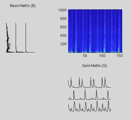
In much the same way that we can factor a number into it's constituent factors (6 = 2 x 3), we can factorize a matrix into two constituent matrices (V = GW, where V, W, and H are all matrices). In this representation, V represents the spectrogram of the input audio, W represents a set of N stationary spectra (spectra is pretty much the FFT), and H represents a set of N volume envelopes (Where N is the number of sources/drums/instrument types present in the recording). Each of the spectra in W is related to a particular volume envelope in H. The combination of a spectra and its corresponding volume envelope represents a single source/drum/instrument. The image below shows the result of a factorization where N = 3. The spectrogram in the upper right is V, the Basis Matrix is W, and the Gain Matrix is H. The first row of the Gain Matrix is the volume envelope for the bass drum, the second row is the volume envelope for a snare drum, and the third row is the volume envelope for a hi-hat (note the wide-band nature of it's spectra in the corresponding Basis Matrix column).

The 'Non-Negative' bit comes from the constraint that no element in V, W or H may be negative. In other words, we can only add up bits of sound, we can not subtract bits of sound in our factorization. The nice bit about this constraint is that it encourages the factorization to be parts-based.

If you're more interested in the mathematics behind NMF, Tuomas Virtanen is a bit of an NMF expert and he has a number of quite nice papers on the subject as it applies to Audio.

There are a number of nice MATLAB implementations of NMF available, chiefly - it seems - because MATLAB comes with all of the necessary data structures and algorithms to easily deal with matrices. C++ is well suited for matrix manipulations, but not out of the box. I'm not a terribly experienced C programmer, but after a bit of research, it seems like the best available options for matrix mathematics are BLAS, LAPACK, Armadillo, and Eigen. I have decided to go with Eigen, mainly because the BLAS/LAPACK libraries have a quite scary interface/syntax, and because of this interview with the Eigen developers.

The Eigen syntax is quite nice if you come from an object-oriented background, and possibly most appealing is the fact that you do not need to build or compile any source when using Eigen; you simply copy some header files into your project, and you are ready to create and manipulate matrices.

The following code implements a version of Virtanen's algorithm in the Eigen C++ library (an appropriate number of iterations/updates is generally something like 300. You can also re-write this sort of algorithm to terminate when the reconstruction error between GW and V is low):

void factorizeMatrix(MatrixXf V_, MatrixXf W_, MatrixXf H_, int num_updates_) {

 

int xSize = V_.cols();

int ySize = V_.rows();

// Create our Gain matrix with randomized initial values

H_ = MatrixXf(num_sources_, xSize);

H_.setRandom();

H_ = H_.array().abs();

// Create our Spectra matrix with randomized initial values

W_ = MatrixXf(ySize, num_sources_);

W_.setRandom();

W_ = W_.array().abs();

// Create an identity matrix

MatrixXf ones = MatrixXf::Constant(xSize,ySize,1.0);

// Run the update rules for numUpdate iterations

for(int i = 0; i < num_updates_; i++) {

// update spectra

MatrixXf WH = (W_ * H_).array() + 0.00001;

MatrixXf numerator = (V_.array() / WH.array());

numerator = numerator * H_.transpose();

MatrixXf denominator = (H_ * ones).array() + 0.00001;

W_ = W_.array() * numerator.array();

W_ = W_.array() / denominator.transpose().array();

// update gains

WH = (W_ * H_).array() + 0.00001;

numerator = (V_.array() / WH.array());

numerator = W_.transpose() * numerator;

denominator = (ones * W_).array() + 0.00001;

H_ = H_.array() * numerator.array();

H_ = H_.array() / denominator.transpose().array();

}

// At this point, you have the relevant spectra and volume envelopes in W and H!

}

Magnitude and Phase of a Complex Number

As a follow-up to the post about the STFT, here are two functions that will come in handy if you are looking to get magnitude or phase information from the complex-valued FFT output. These are similar to the abs() and angle() functions in MATLAB. Note that MATLAB uses the atan2() function as opposed to simply the atan() routine.

Remember that a complex number specifies a vector in the complex plane, so the overloaded nature of abs() in MATLAB can be slightly confusing. What you really want is the magnitude, or length of the vector, which you can get with Pythagoras' theorem.

Check out this link for a nice primer on complex numbers.

// Computes the magnitude of a complex number/vector in the complex plane (similar to abs() in MATLAB)

float computeMag(fftw_complex num) {

double real = num[0];

double imag = num[1];

return sqrt((real * real) + (imag * imag));

}

// Computes the phase of a complex number/vector in the complex plane (similar to angle() in MATLAB)

float computePhase(fftw_complex num) {

double real = num[0];

double imag = num[1];

//SOHCAHTOA

// Tan(@) = imag/real

return atan2(imag, real);

}

Short Time Fourier Transform with FFTW3

For an OpenFrameworks project I was recently working on, I needed a spectrogram, or STFT representation of some audio data. The spectrogram gives you an idea of how the frequency content of a signal changes over time. While the formula may look a little hairy, you can really just think of the STFT as  a process that chops up your signal into chunks, and applies a DFT or FFT to each chunk. When the outputs of each FFT are lined up side by side, you have yourself a spectrogram.

The basic process is as follows:

1) Slice out a chunk of the signal
2) 'window' the chunk*
3) Compute the DFT/FFT of the chunk
4) Store the DFT/FFT output somewhere
5) Slice the next chunk out of the signal**
6) Keep repeating until you hit the end of the signal


* Because of the eccentricities of the DFT and FFT (spectral leakage, etc), the formulation gets a little confused with notions of windowing and other miscellany. The question you might ask, is why we are 'windowing' the chunk, and what does 'windowing' mean? This link will give you the proper answers, I'm sure, but I'll throw out an intuitive answer.

First off, 'windowing' simply means multiplying one signal by another signal. This 'other' signal is known as a window. If our window was an infinitely long series of zeros, the result of windowing would be to completely zero out our signal. If our window was an infinitely long series of zeros save for a single value of 1 at time 0 (also known as an 'impulse'), the result of windowing would be to zero out every element in our signal except for the sample at time 0.

This means that if we slice out a 'chunk' of samples from our signal, we have in strict terms just windowed our signal. For example, if we slice out the first 1024 samples from our signal, we have just windowed our signal with a 'rectangular window'. The first 1024 samples in our rectangular window have a value of 1, and the rest of the window's samples have a value of 0.

Generally, a rectangular window shape is undesirable, as it introduces unwanted frequency content. If you're feeling interested in alternative window shapes and their effect on DFT/FFT calculations, look here. Also, remember the convolution theorem, which states that multiplication in the time-domain is equivalent to convolution in the frequency domain. This should help you intuitively understand why certain window shapes are more or less desirable. For our purposes, we are using a Hamming window, as it is the default window used in the MATLAB STFT/spectrogram routine.  Here is C++ code to create a Hamming window in a float buffer, equivalent I believe, to the MATLAB function hamming():

// Create a hamming window of windowLength samples in buffer

void hamming(int windowLength, float *buffer) {

 for(int i = 0; i < windowLength; i++) {

   buffer[i] = 0.54 - (0.46 * cos( 2 * PI * (i / ((windowLength - 1) * 1.0))));

 }

}

** Each 'chunk' that we slice out of the signal will have the same length (It is wise to choose a length that is a power of two, as FFT routines are optimized to deal with signals whose length is a power of two. You also need to ensure that the length is neither too long, nor too short. For audio applications, it seems like 2048 is usually a good choice. If your chunks are too short, you cannot properly analyze the frequency content of low-frequency signals, and if your chunks are too long, you get poor time localization of frequency analysis. This whole issue actually relates to Heisenberg's Uncertainty Principle!)

Let's assume that we decide to divide up our signal into chunks of 2048 samples. The first chunk will be composed of the first 2048 samples of the signal, or the 0th to 2047th samples.

We now have to decide what samples make up the second 'chunk'. One option is to have no overlap in our chunks, which would amount to taking the 2048th to 4095th samples from our audio file. Another option would be to have lots of overlap in our chunks: we could use the 1st to 2048th samples for the second chunk. In the former case, we say that the STFT has a 'hop size' of 2048 samples (no overlap). In the latter case, we say that the STFT has a 'hop size' of 1 sample (lots of overlap). The 'hop size' can be thought of as the distance between the starting point/index of of successive chunks.

Your choice of hop size depends largely upon the specific concerns of your analysis. If you are looking for a rough, general picture of how the frequency content of the signal evolves over time, a large (little overlap) hop size is probably fine. If you need a very faithful representation, or are interested in re synthesizing the STFT data as audio in the time-domain, you should choose a small hop size. You also need to think about your storage and performance requirements. A small hop size means more DFT/FFT calculations!

Ok, I think that's enough to get the general picture of what's going on. Here is some rough, probably buggy C++ code that implements an STFT routine using the FFTW3 library. It's probably not optimal performance-wise, but might give you a good starting point for writing your own:

void STFT(std::vector <float> *signal, int signalLength, int windowSize, int hopSize) {

    fftw_complex    *data, *fft_result, *ifft_result;

    fftw_plan       plan_forward, plan_backward;

    int             i;

    data        = ( fftw_complex* ) fftw_malloc( sizeof( fftw_complex ) * windowSize );

    fft_result  = ( fftw_complex* ) fftw_malloc( sizeof( fftw_complex ) * windowSize );

    ifft_result = ( fftw_complex* ) fftw_malloc( sizeof( fftw_complex ) * windowSize );

    plan_forward  = fftw_plan_dft_1d( windowSize, data, fft_result, FFTW_FORWARD, FFTW_ESTIMATE );

    // Create a hamming window of appropriate length

    float window[windowSize];

    hamming(windowSize, window);

    int chunkPosition = 0;

    int readIndex;

    // Should we stop reading in chunks? 

    int bStop = 0;

int numChunks = 0;

// Process each chunk of the signal

while(chunkPosition < signalLength && !bStop) {

// Copy the chunk into our buffer

for(i = 0; i < windowSize; i++) {

        readIndex = chunkPosition + i;

        if(readIndex < signalLength) {

              // Note the windowing!

data[i][0] = (*signal)[readIndex] * window[i]; 

data[i][1] = 0.0; 

        } else {

 
             // we have read beyond the signal, so zero-pad it!

data[i][0] = 0.0; 

data[i][1] = 0.0; 

bStop = 1;

}

}

// Perform the FFT on our chunk

fftw_execute( plan_forward );

/* Uncomment to see the raw-data output from the FFT calculation

std::cout << "Column: " << chunkPosition << std::endl;

for(i = 0 ; i < windowSize ; i++ ) {

fprintf( stdout, "fft_result[%d] = { %2.2f, %2.2f }\n",

i, fft_result[i][0], fft_result[i][1] );

}

*/

// Copy the first (windowSize/2 + 1) data points into your spectrogram.

// We do this because the FFT output is mirrored about the nyquist 

// frequency, so the second half of the data is redundant. This is how

  // Matlab's spectrogram routine works.

for (i = 0; i < windowSize/2 + 1; i++) {

yourDataStructureGoesHere = fft_result[i][0];

yourDataStructureGoesHere = fft_result[i][1];

}

chunkPosition += hopSize;

numChunks++;

} // Excuse the formatting, the while ends here.

fftw_destroy_plan( plan_forward );

fftw_free( data );

fftw_free( fft_result );

fftw_free( ifft_result );

}

Installing FFTW3 with xcode and OpenFrameworks

Moving on from loading audio files with libsndfile (here and here), you'd probably like to perform some frequency domain analysis using Fourier transforms (that's a good video if you think of formulas as algorithms). It seems that the best/most popular library for FFT implementations is the FFTW3 library.

Installation of FFTW3 is very similar to the installation of libsndfile, in that you need to use macports (or homebrew) to install a universal build of the library for use with OpenFrameworks. As discussed earlier, a 'normal' install will most likely build an X86 64-bit library, where we need a 32-bit i386 library build.

Assuming you are using macports, type this into a terminal window:

> sudo port install fftw-3 +universal

Aside - A handy trick for seeing which architecture your library is built for is to use the 'lipo' command. Navigate to the folder where your library lives, and type this into a terminal window:

> lipo -info libfftw3.a

Anyways, the port install command will place the fftw3.h header file in your_HD/opt/local/include folder, and the libfftw3.a library in your_HD/opt/local/lib folder. To use the library in your OF project, add these two files to your project via the menu option Project -> Add to project...

Now, you can include the library in your source by adding the following include statement:

#include "fftw3.h"

The FFTW3 documentation is very thorough, but if you'd like some boiler plate code to see how to calculate a simple FFT, it can be hard to come by. As a warning, copy/pasting example code with this library seems pretty dicey as older versions of the library used considerably different syntax. Thankfully, this guy posted some very nice code for testing the operation of the library. I'm reposting it here after some simple explanation:

int SIZE : This is the size or length of the transform. FFTs are designed to work with transform sizes that are a power of 2. In this case, we just transform a simple signal that is 4 samples long that looks like this:

[1.0, 1.0, 1.0, 1.0]

data: This structure holds the data we want an FFT of. The FFTW library is built to allow for transforms of complex data, but audio data is real-valued only (no imaginary component). As such, we will only fill one 'side' of the structure with our real valued samples (check out the first for loop).

When you run this example, you should see the following output in your xcode console (Run->console) if everything is working with your install:

data[0] = { 1.00, 0.00 }

data[1] = { 1.00, 0.00 }

data[2] = { 1.00, 0.00 }

data[3] = { 1.00, 0.00 }

fft_result[0] = { 4.00, 0.00 }

fft_result[1] = { 0.00, 0.00 }

fft_result[2] = { 0.00, 0.00 }

fft_result[3] = { 0.00, 0.00 }

ifft_result[0] = { 1.00, 0.00 }

ifft_result[1] = { 1.00, 0.00 }

ifft_result[2] = { 1.00, 0.00 }

ifft_result[3] = { 1.00, 0.00 }

You can check the correctness by performing the equivalent commands in MATLAB:

>> data = [1.0, 1.0, 1.0, 1.0];
>> fft(data)
ans = 
4    0    0   0
>> ifft(ans)
1    1    1   1


Here's the example C code:

int SIZE = 4;

fftw_complex    *data, *fft_result, *ifft_result;

fftw_plan       plan_forward, plan_backward;

int             i;

data        = (fftw_complex*) fftw_malloc(sizeof(fftw_complex) * SIZE);

fft_result  = (fftw_complex*) fftw_malloc(sizeof(fftw_complex) * SIZE);

ifft_result = (fftw_complex*) fftw_malloc(sizeof(fftw_complex) * SIZE);

plan_forward  = fftw_plan_dft_1d(SIZE, data, fft_result,
                                 FFTW_FORWARD, FFTW_ESTIMATE);

plan_backward = fftw_plan_dft_1d(SIZE, fft_result, ifft_result,
                                 FFTW_BACKWARD, FFTW_ESTIMATE);

for( i = 0 ; i < SIZE ; i++ ) {

    data[i][0] = 1.0; // stick your audio samples in here

    data[i][1] = 0.0; // use this if your data is complex valued

    }

for( i = 0 ; i < SIZE ; i++ ) {

    fprintf( stdout, "data[%d] = { %2.2f, %2.2f }\n",
    i, data[i][0], data[i][1] );

}

fftw_execute( plan_forward );

for( i = 0 ; i < SIZE ; i++ ) {

    fprintf( stdout, "fft_result[%d] = { %2.2f, %2.2f }\n",

i, fft_result[i][0], fft_result[i][1] );

}

fftw_execute( plan_backward );

for( i = 0 ; i < SIZE ; i++ ) {

    fprintf( stdout, "ifft_result[%d] = { %2.2f, %2.2f }\n",

i, ifft_result[i][0] / SIZE, ifft_result[i][1] / SIZE );

}

fftw_destroy_plan( plan_forward );

fftw_destroy_plan( plan_backward );

fftw_free( data );

fftw_free( fft_result );

fftw_free( ifft_result );

Using ofSoundStream to play arbitrary audio data

If you're looking for the ability to pipe raw audio through OpenFrameworks, and aren't interested in using the built in ofSoundPlayer objects, start here. Grimus has put up some very nice code for what is essentially a framework for loading, playing, and effecting audio in a manner that'll be familiar and easy for those looking to do DSP.


If you just want a bare-bones explanation, I'll give you a little overview here. In your application's setup() method, you need to setup the ofSoundStream with a reference to your application, and some other information like the sample rate:

void testApp::setup(){

 

...

sampleRate = 44100;

lAudio = new float[256];

rAudio = new float[256];

ofSoundStreamSetup(2, 0, this, sampleRate, 256, 4);

...

}

In the above case, we are setting up the ofSoundStream with 2 output channels, 0 input channels, a reference to our application, the sample rate of 44100 hz, a buffer length of 256 samples, and 4 somethings (I forget what the four is for). Once you've done this, your application will periodically be asked to fill a buffer full of audio for output. To ensure that the application can properly respond to this request, you need to implement the following method in your testApp implementation (testApp.cpp or whatever you've called it). Make sure you also update your header file!

void testApp::audioRequested (float * output, int bufferSize, int nChannels){

    for (int i = 0; i < bufferSize; i++){

lAudio[i] = output[i*nChannels    ] = left_channel_sample_goes_here;

rAudio[i] = output[i*nChannels + 1] = right_channel_sample_goes_here;

    }

}

At this point, you are now responsible for filling up 256 (as defined above for the buffer size) samples of audio output every time the method is called. We save the outputted audio in the lAudio and rAudio buffers in case we'd like to graph the output or do something else nifty with recent output.

That's all there is to it!

Loading a wav File with SndfileHandle

Assuming you have libsndfile installed and properly building with your project (check here), it is time to read some audio from disk into an array. I think it's most convenient to use the C++ wrapper class 'SndfileHandle' defined in the sndfile.hh include as shown below:

#include "testApp.h"

#include <sndfile.hh>

#include <stdio.h>

void testApp::setup(){

.

.

.

const char* fn = "/Users/.../test.wav";

SndfileHandle myf = SndfileHandle(fn);

printf ("Opened file '%s'\n", fn) ;

printf ("    Sample rate : %d\n", myf.samplerate ()) ;

printf ("    Channels    : %d\n", myf.channels ()) ;

printf ("    Error       : %s\n", myf.strError());

printf ("    Frames      : %d\n", int(myf.frames())); 

puts("");

 static float buffer [1024]; 

 myf.read (buffer, 1024);

.

.

.

Aside - The 'frame' terminology initially confused me, as I tend to think of 'frames' as being chunks of multiple samples across the time axis (as in STFT analysis). In the libsndfile world however, a 'frame' is all of the values/samples for each channel at a given time instant. For example, if you have a stereo (2-channel) file, a frame will consist of two values or samples. If you have a mono (1-channel) file, a frame will consist of only one value or sample.

It's fairly non-obvious what is actually stored in our float buffer after the call to the SndfileHandle read() method. if you were dealing with MATLAB, you'd have a 2-dimensional array with each column holding the samples for either the right or left channel after a similar call to wavread(). You might even think it would make more sense for the read() method to return the samples corresponding to each channel separately. However, the read() method implemented in libsndfile fills up a 1-dimensional array of values.

For a mono (1-channel) audio file, the interpretation is simple. The buffer is filled with the audio samples just as you might expect:

buffer = [sample1, sample2, sample3, sample4, etc]

For a stereo (2-channel) audio file, the interpretation is less obvious. The buffer is filled with the audio samples in an interleaved fashion:

buffer = [left_sample1, right_sample1, left_sample2, right_sample2, etc]

This pattern continues for n-channel multichannel files.

If you want to inspect the contents of 'buffer' by hand, place a breakpoint after the read() function (double click in the wide column to the left of the text. A little blue tab/flag should appear). Next, go to Build -> Build and Debug, and wait until your program halts at the breakpoint. Now, go to Run -> Show -> Expressions. Enter the following in the the text field at the bottom of the dialogue:

*buffer @ 1024

Hopefully any newcomers to libsndfile and xcode will find this useful!